Let Sino's Lamination Stacks Empower Your Project!
To speed up your project, you can label Lamination Stacks with details such as tolerance, material, surface finish, whether or not oxidized insulation is required, quantity, and more.
Most of the error in motor core-loss prediction is locked in long before meshing or solver settings. It sits in three quiet choices: what you accept as a BH curve, how you massage core-loss data into coefficients, and how those two sets of numbers meet inside your FEA tool. Get that pipeline mostly right and even a plain model is workable; get it wrong and no refinement trick will rescue the watts per kilogram.
Let’s skip definitions. You already know hysteresis, eddy, excess, rotation, DC bias. The more useful question is: what total error on stator and rotor iron loss is tolerable for your project. Ten percent? Twenty?
Recent comparisons of iron-loss models in machines show that changing only the loss model or coefficients, with exactly the same FEA fields, can swing predicted losses by tens of percent over the operating map. That is before you argue about mesh, skew, or 3D effects. So the materials pipeline deserves the same design effort you’d give to the rotor topology.
If the spec says “efficiency within one percentage point” and iron loss is a big slice, then that target quietly implies constraints on your bh data quality, your fitting method, and your extrapolation habits. Otherwise you’re tuning in the dark.
On paper you want: a clean anhysteretic BH curve over the full flux range, resolved core-loss data vs B and f for your exact lamination thickness, plus temperature dependence and processing effects. In practice you get something else. Usually a DC or low-frequency BH curve and a handful of total loss points from Epstein or SST tests at catalog frequencies.
The gap between “want” and “have” is where your FEA setup lives. The table below is a simple way to make that gap explicit.
| Aspect | What you usually have | What your FEA actually wants | Comment |
|---|---|---|---|
| BH curve type | DC or low-frequency major loop; maybe one AC BH curve | Single-valued BH (often anhysteretic) over full B range | Using dynamic BH directly can double-count losses if you also use a loss model |
| Flux-density range | Up to roughly 1.7–1.8 T, sometimes less at high frequency | At least up to worst-case tooth tip flux plus margin | Extrapolation method matters more than it looks |
| Frequency coverage | 50/60 Hz and a few higher points (100–400 Hz) | From near-DC behavior to your maximum equivalent frequency | Needed whether you use Steinmetz, Bertotti or look-up tables |
| Loss data format | W/kg vs B for several fixed frequencies | Either fitted loss-model coefficients, or loss vs B and f on a grid | FEA codes rarely work directly with the raw catalog curves |
| Processing / stress info | Sometimes: “fully processed” vs “as punched” | Loss data that matches the actual stamping and assembly process | Cutting can easily add 20–50% to loss around slots |
| Temperature dependence | Maybe one curve at 23 °C | Loss model valid over your thermal envelope | Coefficients drift with temperature; many fits silently ignore this |
Once you write this down for your project, “core-loss setup” stops being an abstract step. You see the missing pieces. You also see which compromises you’re making deliberately, instead of by default.
There is no single correct iron-loss model for every machine, but there is such a thing as a coherent story. You only need one. A typical chain goes like this.
You choose a loss-separation style model (Steinmetz family, Jordan, Bertotti-type) or a hysteresis model plus dynamic corrections. You extract coefficients from measurement data or supplier curves. You run FEA to get B(t) in each element. You integrate the loss model on that waveform. Done. At least on paper.
That chain breaks when the BH curve you feed into FEA already contains dynamic effects that your loss model assumes are separate. Or when your Steinmetz coefficients are fitted in a narrow, low-frequency window but you use them for high-frequency PWM excitation. Or when your material data reflects Epstein samples, while your machine core is stamped, shrunk, welded and stressed in ways the catalogue never saw.
So first decision, in plain terms:
You either let the FEA solver carry only the quasi-static BH nonlinearity and keep all dynamic loss in a separate model, or you bring some form of hysteresis and dynamics inside the material model and reduce what the external loss model has to cover. Mixing both halfway is what generates the noisy, hard-to-trust numbers.
Most commercial FEA codes want a single-valued BH relationship. They can handle nonlinearity, but not an explicit hysteresis loop at every integration point. The usual workaround is to feed an anhysteretic or “effective” BH curve that approximates the core’s average magnetization behavior.
You rarely get that curve directly. So you assemble it.
A practical scheme is to take low-frequency or DC data as the backbone, clean up noise, and extend it to your operating flux levels. High-frequency AC BH data, when available, is useful mainly to check saturation behavior and to avoid ridiculous extrapolations above the knee. If you use AC BH directly as your material curve and then apply a loss model on top, you’re counting some loss terms twice.
Above the measured range you have to extrapolate. The blunt method is to force the curve towards a horizontal asymptote at the material’s estimated saturation induction, derived from density and resistivity correlations. It is not subtle, but it’s better than allowing the solver to operate in a regime where the BH slope accidentally increases again due to poor fitting.
Temperature is awkward. Most BH curves are measured near room temperature, while machines run hotter. Saturation level drops and coercivity changes with temperature; Steinmetz-type coefficients do too. If your FEA tool supports temperature-dependent material sets, link them; if it does not, at least check that your chosen BH curve still gives realistic current and power factor at rated temperature when compared to tests. Even approximate scaling is safer than pretending that 20 °C and 120 °C are equivalent.
Finally, remember that machining and assembly modify the effective BH curve, not just the loss curve. Slotted cores show different magnetization behavior than flat samples. You can either embed that into an “effective BH” from back-calculation versus test, or leave BH pristine and inflate loss coefficients. Doing both again leads to double counting.
Most FEA environments ask for loss model coefficients: hysteresis, eddy, maybe excess. These are not magical constants; they are the end result of a curve fitting exercise against measured W/kg vs B and f.
The basic recipe is simple. Convert catalog curves into data points, linearize appropriately (log–log or with the usual Ps/(B²f) vs f trick), and run regression to extract coefficients. The part that makes or breaks accuracy is everything you decide around that fitting step.
One decision: whether you treat all frequencies as equal during fitting. If your machine spends most of its life near one frequency band, weight that region more heavily in the error function. The literature is clear that Steinmetz-type coefficients drift with frequency; forcing a single set to match both 50 Hz and high-frequency conditions without any weighting often gives mediocre predictions everywhere.
Another: whether you fit separate coefficient sets per region of the machine (teeth versus yoke, stator versus rotor). The physics does not change by region, but the effective behavior does once you include local stress, different lamination batches, and manufacturing details. Some recent PMSM studies show that the apparent coefficients required to match measured losses in teeth and yoke can differ noticeably, even for the same nominal grade. That is not elegant, but it is observable, and your FEA setup can exploit it.
Motors almost never operate on perfect major hysteresis loops. There are minor loops everywhere: light-load conditions, partial magnetization, local demagnetization under slots. Old papers and newer work both show that ignoring minor loops can under- or over-estimate hysteresis loss substantially, especially with non-sinusoidal excitation.
Several paths exist. One is to keep a straightforward loss-separation model but correct for minor loops through empirical factors or energetic models derived from quasi-static loop measurements. Another is to use explicit hysteresis models (Jiles–Atherton, Preisach, Play model) behind the scenes, letting them regenerate local loops from measured symmetric BH data. These approaches are heavier to set up, but they free you from having to measure loss curves under every possible waveform.
DC bias and rotational fields are similar stories. Works on rotational magnetization show that losses at tooth tips and junctions can be significantly higher than those predicted assuming purely alternating flux. Newer FEA-based methods introduce rotational correction factors or separate loss terms, while others model rotation directly by post-processing local B and H waveforms.
So the choice is less “should I model rotation and DC bias” and more “how much approximation is acceptable given my operating space”. If you are designing a high-speed machine with strong spatial harmonics, not accounting for rotation at all is a design assumption, not just a simplification.
Once BH and loss coefficients exist somewhere on your server, they still need to be expressed in the dialect of your chosen FEA tool. Different codes expect different ingredients. Some want only BH and a Steinmetz triplet. Others want full BH plus frequency-dependent loss tables. Yet others have built-in hysteresis options if you give them symmetric BH loops and electrical conductivity.
A few practical patterns tend to work across tools.
Treat the BH curve as geometry-independent. You should not be changing BH by region just to match global torque or current; that is calibrating away deeper problems. At most, you can choose different material cards when the manufacturing route really differs, for example, stress-relieved rotor versus heavily punched stator.
Treat loss coefficients as geometry-dependent if needed. It is acceptable to keep the same BH but use slightly different effective hysteresis or excess coefficients in teeth and yoke, reflecting different stress and cutting damage, provided these differences are supported by measurements or at least by literature ranges.
Keep solver settings boring at first. Time step, harmonic order, and mesh refinement all interact with local waveform quality and thus with loss prediction. Before tweaking them, verify that, with a conservative setup, your post-processed FEA losses at one or two standard operating points are at least in the same band as measurements using your current material data. If you are off by a factor of two, this is almost never a meshing issue; it is almost always material data and model mismatch.
There are a few checks that cost less than another optimization run and expose issues in the material setup rather than in the geometry. Rough but efficient.
Compare your fitted loss model back against the original Epstein or SST curves across all available frequencies. Do this before you even touch FEA. If you see systematic over- or under-estimation at high flux density, now you already know how your FEA result will be biased in heavy-load conditions.
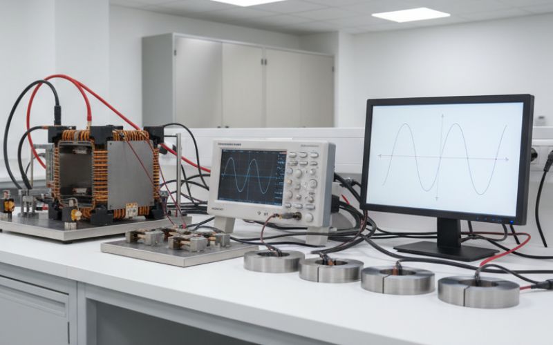
Feed the same BH and loss model into a simple 2D test geometry, something close to the standardized single-sheet or toroidal core setup, and compare predicted loss against the published data or your own lab measurement. Many recent works use that loop—measurement, FEA of the measurement setup, coefficient correction—to clean up BH and loss curves before using them in machines.
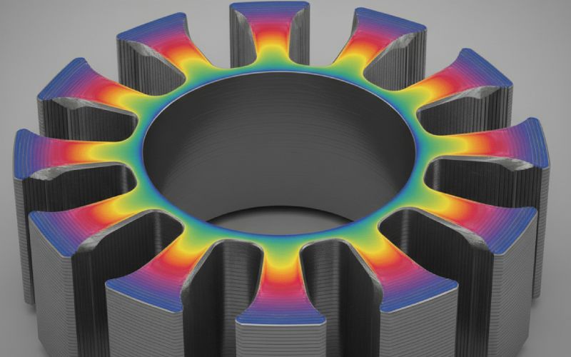
Inspect element-wise loss maps at several operating points. If the distribution does not match what you expect physically—loss concentrated at tooth tips, yoke corners, bridge regions under high harmonic flux—this is often a sign that your BH curve or loss model is not correctly capturing saturation or rotational effects. Studies on high-frequency machines and mixed-grade cores show very clear spatial patterns; your model should at least roughly mimic them.
Finally, accept that some calibration is unavoidable. Even very detailed frameworks grounded in measurements of electrical steels and advanced hysteresis modeling still report noticeable spread between models and hardware under complex waveforms. Calibration is not a failure of physics; it is an admission that the material in your machine is not the same as the coupon in the catalog.
The short version is simple. Treat BH curves and core-loss data as design parameters, not as background constants. Decide your loss-model story, build a BH curve that matches it, fit coefficients to the data you actually have, and then use FEA as the calculator that sits on top of those choices.
Do that, and core-loss prediction stops being a mysterious number the software prints at the end. It becomes just another approximation, with known assumptions and controllable error, that you can argue about and improve on the next design.